How Stable Diffusion works
Understand in a simple way how Stable Diffusion transforms a few words into a spectacular image.
Introduction
To use Stable Diffusion it is not necessary to understand how it works, but it helps. Many configurable parameters like Seed, Sampler, Steps, CFG Scale or Denoising strength are essential to generate quality images.
In this article we are going to see, in broad strokes, without a single line of code and almost for everyone, how Stable Diffusion works internally in its version 1.x and how it is able to generate such creative images with a simple text sentence.
I have published a second part of this article. In this new article we will implement Stable Diffusion 1.5, using Python code. Since here we will see the theory behind image generation, in the second part we will put it into practice and see how the pieces are interconnected with each other. It's not because I say so, but it is an ideal complement to this article.
How a diffusion model works
Within machine learning there are several types of generative models (models capable of generating data, in this case images). One category is diffusion models and they are so called because they imitate the behavior of molecular diffusion. A phenomenon that we have all experienced when using air freshener or pouring ice into a glass of water. The particles tend to move and spread.
Forward diffusion
The Stable Diffusion training starts with hundreds of thousands of photographs taken from the Internet and begins by adding Gaussian noise to the images over a series of steps until the images lose all meaning. In other words, noise is diffused in the images in the same way that an air freshener diffuses its particles in a room. This process is known as forward diffusion (since it goes forward).
Reverse diffusion
When we ask Stable Diffusion to generate an image, the magic known as reverse diffusion happens, a process that reverses the one seen previously.
The term inference is also used when putting into practice what a model has learned during training. In the case of Stable Diffusion this term can be used for the reverse diffusion process.
The first step is to generate a 512x512 pixel image full of random noise, an image without any meaning. To generate this noise-filled image we can also modify a parameter known as seed, whose default value is -1 (random). For example, if we use the seed number 4376845645 the same noise will always be generated, hence the result of an image can be replicated if we know its seed.
Then, to convert an image full of noise into a dog in a Batman costume and reverse the process, you have to know how much noise is in the image. This is done by training a convolutional neural network to be able to predict the level of noise within an image. This model is called U-Net (or denoising U-Net), although in Stable Diffusion it is known as noise predictor.
The training of this model consists of using the images of the forward diffusion process, also indicating how much noise we have added so that it is capable of learning it. If I tell you that the first image has 0% noise, the middle one 50% and the last one 100%... surely you would be able to distinguish the existing level of noise in a new photograph because you have understood the pattern. Maybe not perfectly but hey, you are not a neural network!
Sampling
With this initial image full of noise and a way to calculate how much noise is still left in the image the sampling process begins.
The noise predictor estimates how much noise is in the image. After this, the algorithm called sampler generates an image with that amount of noise and it is subtracted from the original image. This process is repeated the number of times specified by steps or sampling steps.
Examples of sampling algorithms are Euler, Euler Ancestral, DDIM, DPM, DPM2 or DPM++ 2M Karras. The difference is that some are faster, some are more creative, some refine small details better, etc. More information about these algorithms, their uses and differences, in the article Complete guide to samplers in Stable Diffusion.
After repeating this process as many times as necessary we will obtain our final image.
Another important piece of sampling is the noise scheduler as it has the function of managing how much noise to remove at each step. If the noise reduction were linear, our image would change the same amount at each step, producing abrupt changes. A negatively sloped noise scheduler can remove large amounts of noise initially for faster progress, and then move on to less noise removal to fine-tune small details in the image. This algorithm can be configured and chosen from multiple options.
But... how does the model know that there is a dog behind the noise? The answer is that it does not. So far we have managed to generate an unconditioned image. The result can be a car or anything because our prompt is not conditioning the result.
Conditioning
The interesting thing, of course, is not to generate meaningless random images, but to condition the result at each step.
If we recall, we have trained the noise predictor by giving it two things: the image and the level of noise. Therefore we can steer the noise predictor towards the result we want. It's like asking "what is the level of noise in this photograph of a dog in a Batman costume?", instead of simply asking "what is the level of noise?". In the first way we condition the result.
Don't think about a pink elephant!
Using text (prompt) is not the only way to condition the noise predictor. Several and even multiple methods can be used at the same time. Let's look at some examples starting with the most important one.
Text-to-Image
Converting text to a conditioning is the most basic function of Stable Diffusion. It is known as Text-to-Image and consists of several pieces that we will see below.
Tokenizer
Since computers do not understand letters, the first task is to use a tokenizer to convert each word into a number called a symbol (token).
In the case of Stable Diffusion the tokenization is done thanks to the CLIP model (Contrastive Language-Image Pre-Training). This model created by OpenAI converts images into detailed descriptions, although only the built-in tokenizer is used for this task.
The tokenizer does not always convert each word to a token. There may be compound words and space character also affects the number of tokens.
You may have seen somewhere that the maximum number of words a prompt can have is 77. This limitation exists because tokens are stored in a vector that has a size of 77 tokens (1x77). Therefore, this limitation actually refers to tokens, not words. And while it is true that after 77 tokens the rest are discarded, currently other concatenation and feedback techniques are used to condition the noise predictor with as many blocks of 77 tokens as necessary until all of them are used.
This step is the only one exclusive to Text-to-Image, from now on all the conditioning we will see later uses the following layers.
Embedding
Now we are going to carry out an exercise of imagination. We have 10 photographs of people and we have to classify them in a two-coordinate graph based on two parameters: age and amount of hair. If we do the task correctly we will obtain something like the following:
The graph contains two dimensions (X and Y) to represent the groups.
Well, this is an embedding itself. A way of classifying terms and concepts by storing the data in vectors. In the case of Stable Diffusion, a version of CLIP called ViT-L is used which contains 768 dimensions. It is not possible to know what these dimensions are because they depend on the training data, but we could imagine that one dimension is used to represent the color, another for the size of the objects, another for the texture, another for the facial expression, another for the luminosity, another for the spatial distance between objects... and so on up to 768.
Embeddings are used because once the terms have been categorized in dimensions, the model is able to calculate the distance between them.
Using this technique, the dimension that groups the concept of clothing will be closer to the dimension that stores values such as man and woman, than to the dimension that groups the parts of a room such as window or door. This example is quite simple, in reality everything happens in a much more abstract way.
It is worth noting that each token will contain 768 dimensions. That is, if we use the word car in our prompt, that token will be converted into a 768-dimensional vector. Once this is done with all the tokens we will have an embedding of size 1x77x768.
In this way we can measure the distances of all the dimensions of all the tokens.
Transformer
This is the last step of the conditioning. In this part the embeddings are processed by a CLIP transformer model.
This neural network architecture is composed of multiple layers and is in charge of conditioning the noise predictor to guide it in each step towards an image that represents the information of the embeddings.
In Text-to-Image the embeddings are called text embeddings for obvious reasons, but the transformer model can obtain embeddings from other conditioning as we will see a little further down.
Here comes the interesting part of the transformer. It is known as self-attention when all embeddings have the same weight and affect the result equally. In addition to this architecture, within these layers Stable Diffusion also uses cross-attention. This technique consists of calculating the dependency relationships between the embeddings and producing a tensor with the results. This is where the distances between dimensions are taken into account.
For example if we use the prompt a red wall with a wooden door, a self-attention only architecture could generate a wooden wall with a red door. This is totally valid but possibly incorrect.
Thanks to the cross-attention, the model calculates the distance between wood/door and between wood/wall and knows that the first option is more likely/closer. We do this every day, if I tell you to think of a red car you are probably thinking of a sports car, a Ferrari perhaps, not a Toyota Prius. This is because in our brain the words car and red are closer to Ferrari than Prius. This technique is known as attention because it mimics the cognitive process we experience when we pay attention to certain details.
Using this information, the noise predictor is guided to get closer at each step to an image that contains the most probable structure given a conditioning.
Class labels and the CFG Scale value
This other conditioning is important because it helps the transformer by using class labels.
When training a Stable Diffusion model, an external classifier (CG - classifier guidance) is used. This is a model that is responsible for assigning labels to the training images. Thus, the photographs of dogs will have the labels animal and dogs associated, while photographs of cats will have the labels animal and cats (among many others).
When we use a high value in the CG scale, we are asking the transformer to separate the labels that are not similar and focus on the ones that are. On the other hand, with a low value, it is as if the labels were brought closer and when asking for a photograph of a cat, we could obtain the photograph of any other animal (or any other nearby label).
To avoid having to use an external classifier model and thus reduce difficulty during training, the process was improved with a technique called classifier-free guidance (CFG). This means that the guidance no longer needs a classifier model to add labels to the images. During Stable Diffusion training, the image description is used to automatically adjust the classes.
By adjusting the CFG Scale parameter we can demarcate more or less the territory of the labels that we want to use to generate the image. This is why it is often said that this value adds or removes generation freedom. The higher the value, more fidelity because the labels will be carefully selected. The lower the value, more freedom so that Stable Diffusion can generate something that, although not as faithful to our prompt, can achieve higher quality by not having so many limitations.
In my experience the optimal value is between 5.5 and 7.5, although sometimes it is necessary to raise or lower it (especially increase it when the prompt is not respected).
Image-to-Image
If an image is used to condition the result we will be applying Image-to-Image.
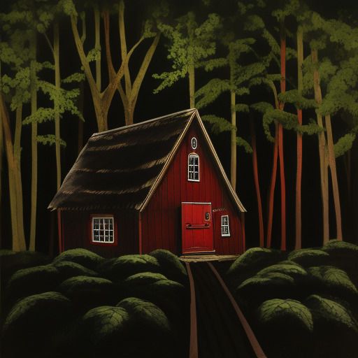
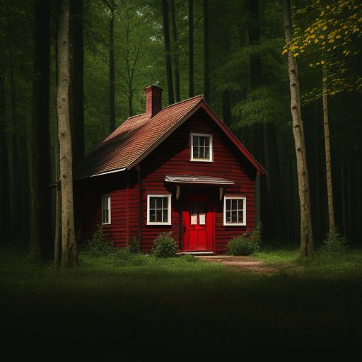
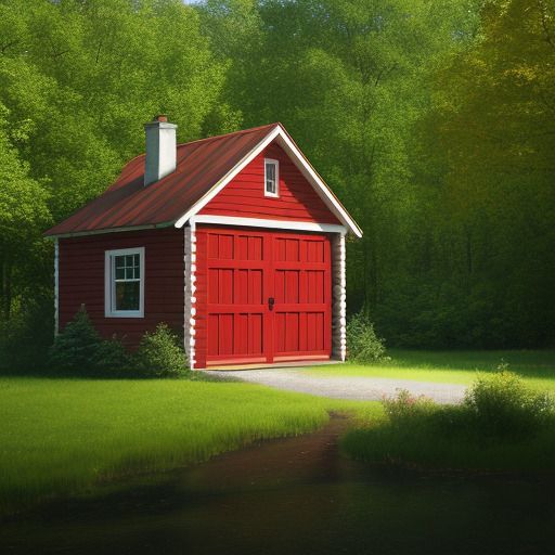
For example, we are going to draw a house in the most sloppy way possible and we are going to pass to Stable Diffusion both this image and the prompt: a realistic photograph of a wooden house with a red door in the middle of the forest. These two conditionings will be applied and we will obtain the following result.
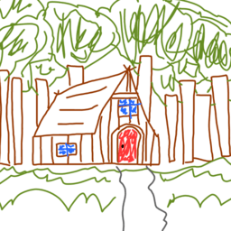

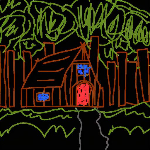
How has it been possible? Well, remember how Stable Diffusion first creates a noise-filled image to work on? Well, instead of this, a certain amount of noise is added to our starting image and we already have the base.
Thanks to the Denoising strenght parameter we can control how much noise we want to add. If we use a value of 0 no noise will be added and therefore we will get an image identical to our sketch. On the other hand, with a value of 1 we will turn our conditioning into pure noise and the sketch will no longer affect the result (it would be like going back to Text-to-Image). Somewhere in between is the ideal value, it depends on how much freedom we want to give Stable Diffusion to respect our input or not.

Inpainting
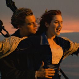
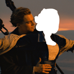
The Inpainting technique in which we can regenerate an area of the image is an Image-to-Image applied to a specific area.

Outpainting
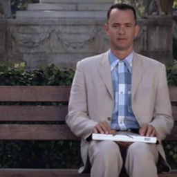
Similarly, the Outpainting technique on which we extend an image by creating new areas that did not exist before, consists of conditioning the noise predictor with several layers. Generally noise is used for the new zone (since it is empty), the prompt and also part of the original image (or all).
Depth-to-Image
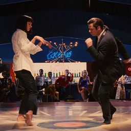
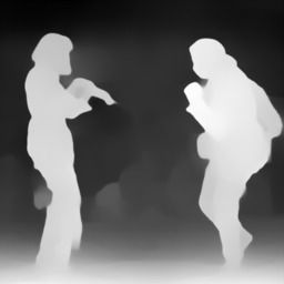
To use the three-dimensionality information of an image, a depth map is used. This technique is known as Depth-to-Image.
A model such as MiDaS processes the image to extract a depth map. Noise is then added depending on the Denoising strenght value and this information is converted to an embedding. Together with the other embeddings the result is conditioned.
In the following example we will use the depth map of an image (the original image is only used to extract the depth map), together with the prompt: two astronauts dancing in a club on the moon.

Other
ControlNet is a neural network that uses a series of models to condition the output in many different ways. It is capable of applying depth maps and poses among many other conditionings.
The following example illustrates pose conditioning using the prompt: astronaut on the moon.


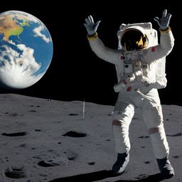
You don't need to extract the pose from an image using OpenPose, you can create it from scratch. For example, through this online editor.
The latent space
There is a missing piece of the puzzle that without it none of this could be done. Throughout this process we have been working on the pixels of the image, this is known as image space. With an image of 512x512 pixels and RGB colors we would have a space of 786432 dimensions (3x512x512), something that you could not run on your home computer.
The solution to this is to use latent space, hence latent diffusion model (LDM). Instead of working on such a large space, it is first compressed to a latent space that is 64 times smaller (3x64x64).
You may be wondering how it is possible to compress the information of an image into something 64 times smaller without losing detail. This is possible because we don't need all the information. It is common for a photograph of a person to show a face, two eyes, a nose, a mouth, etc. Instead of storing all the information of an image, it works with common and relevant features to represent the image in the most efficient way possible. This information is stored in the form of numbers in a tensor of size 3x64x64.
A variational autoencoder (VAE) is a type of neural network that converts an image into a tensor in latent space (encoder) or a tensor in latent space into an image (decoder).
All the processes we have seen in the reverse diffusion technique take place in latent space. This changes the process at two points:
- At the beginning of the process, instead of generating a noise-filled image, latent noise is generated and stored in a tensor. In the case of inpainting, this tensor with latent noise is generated by passing the image through the VAE encoder and then a transformation is applied to the tensor to add the desired noise.
- At the end of the process, when Stable Diffusion has the final result in latent space, the tensor goes through the VAE decoder to become a 512x512 pixel image.
Stable Diffusion also allows you to configure which VAE to use. Depending on the task some offer better results than others, since some information is actually lost in latent space and the VAE is responsible for its recovery.
Stable Diffusion and its versions
Version 1.x of Stable Diffusion is the one we have seen in this article. The difference from model 1.4 to model 1.5 has been the training time, so version 1.5 is capable of generating higher quality images.
In Stable Diffusion 2.x there have been more substantial changes. Version 1.x uses the CLIP ViT-L model from Open AI while Stable Diffusion 2.x uses the OpenCLIP ViT-H model from LAION. This model is a larger version of CLIP ViT-L and has been trained with copyright-free images. Images up to 768x768 pixels have been used as opposed to 1.x which uses images up to 512x512, so images generated with version 2 have higher quality/resolution.
As for copyright-free images, it is positive for the community but has also brought some criticism. The results in some cases are of worse quality than in the previous version when generating images using proprietary styles or celebrity faces. NSFW images are also not allowed in this version.
In version 2.1 the NSFW filter has been relaxed a bit during training, so this type of image can now be generated.
The new SDXL 1.0 version that will be released in July 2023 will be distributed in 2 models: the base model and a new one called refiner. Both have used images with a resolution of up to 1024x1024 with different aspect ratios. The base model uses 2 models for text encoding: OpenCLIP ViT-bigG from LAION and CLIP ViT-L from Open AI. As for the refiner model, it only uses the OpenCLIP model and has also been trained to refine small details, so its use is image-to-image oriented. Both models offer much higher quality than their previous versions, as well as better fidelity of the prompt. Added to this is the fact that they are working with the community so they can optimally train and tune the model to create very high quality derived models (as was achieved with SD 1.5).
Conclusion
To conclude let's recall the main steps of the inference process in Stable Diffusion:
- A tensor with latent noise is generated based on a fixed or random seed. In the case of Inpainting an image is used as a base.
- The conditionings (such as text, depth maps or class labels) are converted to embeddings vectors that store their features in multiple dimensions.
- These vectors go through the CLIP transformer that is responsible for calculating the relationships between the embeddings and their features using the cross-attention technique.
- The noise predictor (U-Net) starts the denoising process using the result of the transformer as a guide to the desired result. This process uses the sampling technique and repeats as many times as the specified number of steps.
- In this process, noise is generated by the selected sampler algorithm and subtracted from the initial tensor. This cleaner noise tensor serves as the basis for the next step until all steps are completed. The noise scheduler controls the amount of progress at each step so that it is non-linear.
- When the denoising process is finished, the tensor leaves the latent space through the VAE decoder, which is in charge of converting it into an image and thus surprising us with the result.
Remember that you can continue in the second part: How to implement Stable Diffusion.
You can support me so that I can dedicate even more time to writing articles and have resources to create new projects. Thank you!